| |
 |
| |
 |
| 1 Cases where Cylindrical Coordinate System is Useful |
| 2 Heat Conduction Equation in Laplacian |
| 3 Heat Flow in a Microscopic Volume |
| 3-(1) Radial Heat Equilibrium |
| 3-(2) Angular Heat Equilibrium |
| 3-(3) Heat Equilibrium in z Direction |
| 3-(4) Overall Heat Equilibrium |
| 4 Summary of Heat Conduction Equations |
| 5 Treatment of Singularity r=0 (Central axis) |
| 6 Differential Expression (See FDM for Detail.) |
| 7 Simulation (See Simulation for Detail.) |
| |
 |
| 1 Cases where Cylindrical Coordinate System is Useful |
| |
| The heat conduction equation in Laplacian can be applied to all coordinate systems. It seems appropriate to use cylindrical coordinate system for round shape materials and products such as round steel bars (billets) and pipes. |
| |
 |
| 2 Heat Conduction Equation in Laplacian |
| |
| The heat conduction equation in Laplacian is as follows. |
| |
 |
| |
| |
| In cylindrical coordinate system, the above formula becomes as follows. |
| |
 |
| |
| It is ok if you can uses the formula; however, the author would suggest to understand how to derive it, because it will become easier to accept and to remember it. Let's derive the heat conduction equation from the flow of heat. |
| |
 |
| 3 Heat Flow in a Microscopic Volume |
| |
| The volume in cylindrical coordinate system of the microscopic one is as follows. |
| |
 |
| |
| Let's omit the fourth power term, because it is negligible small in the volume. And then, the formula of volume can be expressed almost in the same way as Cartesian coordinate system. |
| |
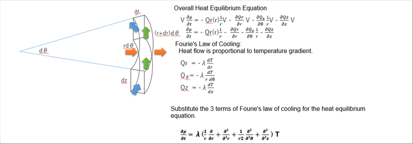
| The arrows in the pictures show the energy flows. Then, we can apply the Fourie's law of cooling. (Fourie's law of cooling: Heat flow is proportional to the temperature gradient.) |
| |
 |
| |
| Please note that the rate of temperature change is the rate of change with respect to distance. Therefore, the denominator of the angle direction is bit different from the r-direction and z-direction. |
| |
 |
| 3-(1) Radial Heat Equilibrium |
| |
 |
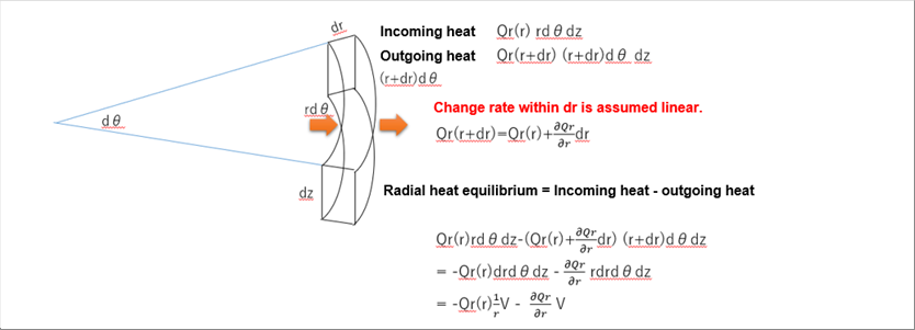
| |
| Since it is a microscopic volume, the heat change in thermal energy is assumed to be proportional to the distance within the volume. (It is assumed that there is no complex relationship of quadratic or higher order.) |
| |
 |
| 3-(2) Angular Heat Equilibrium |
| |
 |
| |
| Since it is a microscopic volume, the heat change in thermal energy is assumed to be proportional to the distance within the volume. (It is assumed that there is no complex relationship of quadratic or higher order.) |
| |
 |
| 3-(3) Heat Equilibrium in z Direction |
| |
 |
| |
| Since it is a microscopic volume, the heat change in thermal energy is assumed to be proportional to the distance within the volume. (It is assumed that there is no complex relationship of quadratic or higher order.) |
| |
 |
| 3-(4) Overall Heat Equilibrium |
| |
| The following picture is a combination of all three energy equilibrium equations. |
| |
 |
| |
| āiāuāēēēÄZÄqéÄgéżéŲüAÆ╝īŹ└ĢWéÓē~ÆīŹ└ĢWéÓō»éČÄ«é┼üAé®é┬Ŗ╚Ģųé╔Ģ\ī╗é┼é½é▄éĘüB |
| |
 |
| 4 Summary of Heat Conduction Equations |
| |
 |
| |
| Apply the differential formula (fg)' = f'g + fg' to the first and second terms comes to the following equation. |
| |
 |
| |
| Since the energy density is Heat capacity times temperature, the following formula is convenient of the temperature simulation. |
| |
 |
| |
| Here, alpha is the coefficient called thermal diffusivity (thermal diffusion coefficient). |
| |
 |
| 5 Treatment of Singularity r=0 (Central axis) |
| |
| In cylindrical coordinate system, the central axis is the singularity. According to references, the singularity can be avoided by approximating with an ellipse instead of a circle; however, the author will omit that here. |
| |
| Mathematically, the central axis is a singular line, but in practice, we can consider that we can safely ignore a small range near the central line, say r is 0.01 and smaller. |
| |
| Let's consider an example oféÆ= 0.01. If the outside diameter is one hundred (100), the area ratio is 0.000001%. The author would suggest not to apply the cylindrical coordinate system if it is a problem. |
| |
 |
| 6 Differential Expression (See FDM for Detail.) |
| |
| The heat conduction equation in cylindrical coordinate system is expressed in central difference form as follow. (See FDM for detail.) |
| |
 |
| |
 |
| 7 Simulation (See Simulation for Detail.) |
| |
| It the temperature distribution at a certain time is known, the temperature change over a minute time later is given by using the above difference equation. So, we can continue calculation in sequence, we will know the necessary temperature distribution at the desired time. |
| |
 |
| |
| If you want to know the temperature distribution in a cross section at a certain location or as a representative of whole body, for example, the author suggest you to omit the z-terms to simplify the formula. |
| |
| Author: T. Oda |
| The page was prepared in Excel, and html and css files were automatically generated by the excel2web. |


